Contour Scanner And Trimmer

Scanning

This tool helps you to find nasty contours which might bug you and prevent your work from being ready for production. It will find open contours, closed contours and self-intersecting contours and checks for a set of other attributes. Bentley-Ottmann algorithm is used to check for those intersections. The algorithm works with the accuracy of the selected paths (epsilons). Self-intersections usually happen if you just have large overlaps where the contour crosses itself like an 'eight' character for example. Using the highlighting it's easy to find contours with unproper path handles. While in a CAD system an area of of a surface can only be calculated if the contour is closed and clean, finding self intersections in Inkscape is not required to do so. SVG format allows to calculate areas on open contours and self-twisted curves. This "artwork behaviour" makes it harder for handling machinery-like drawings for laser cutting, vinyl cutting or whatever. That's why we need to have extra sanity checks but we also have the great freedom of InkScape.

Finding self-intersecting contours does only work for curves with straight line segments (polylines) because it just calculates with a set of given XY points. It does not respect bezier curve segments. Bezier curves have no regular points but special handles, which define the slope of the curve per handle side (left and right). To properly handle a bezier curve we need to split the bezier curve in a lot of small linear lines (acting like infinitessimal solution). We can use the tool "Flatten Bezier to do this by hand or we use the built-in method if Contour Scanner and Trimmer (will make your curve looking edgy or ugly possible). If you want to leave the shape of the line clean (bezier type, no edgy approximation) we can also use Split Bezier (Subdivide) or Add Nodes instead. But remember that your calculated self-intersection points will only be an approximation then. The higher the subdivide count is the higher the precision of the calculated self-intersecting points coordinates will be.

After performing operations, which flatten or split the bezier curve, we we can or should use Chain Paths to put the pieces together again.

Trimming

By having a set of flattened straight line and finding global intersections we can also trim the paths using python library called "shapely". This allows to receive cut segments. Some basic tools to remove duplicates, are integrated.

The result

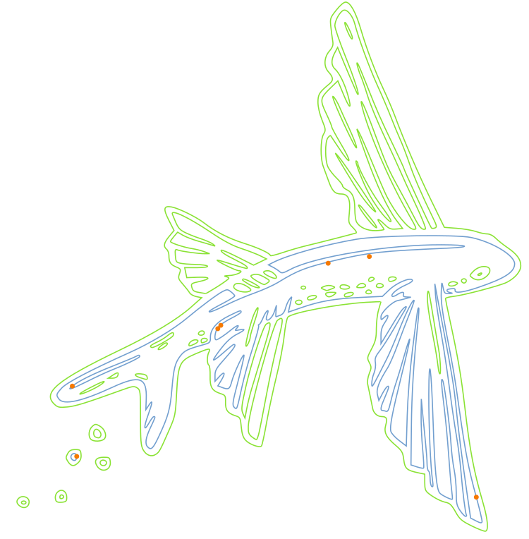
Using Contour Scanner correctly, we get a planar graph style drawing, like the definition gives: "In graph theory, a planar graph is a graph that can be embedded in the plane, i.e., it can be drawn on the plane in such a way that its edges intersect only at their endpoints. In other words, it can be drawn in such a way that no edges cross each other. Such a drawing is called a plane graph or planar embedding of the graph. A plane graph can be defined as a planar graph with a mapping from every node to a point on a plane, and from every edge to a plane curve on that plane, such that the extreme points of each curve are the points mapped from its end nodes, and all curves are disjoint except on their extreme points. " (https://en.wikipedia.org/wiki/Planar_graph)

Tips

• If nothings is selected, the whole document will be processed, regardless of groups. In contrast, if you made a custom selection, check to handle or not to handle groups.

• Works with paths which have Live Path Effects (LPE)

• Convert your strokes and objects to paths before
• Does not work for clones. You will need to unlink them before
• Use extensions to filter short/unrequired paths
• Use extensions to purge or repair invalid paths
• Use 'Path → Simplify' or hit 'CTRL + L' to simplify the trimmed result. With a fine quantization setting the simplified paths will be nearly identical to the original path (except the position of control points)
• Do not select too much paths at once if you have got a fine settings for quantization. This extension is slow and might calculate hours on ultra high configurations.

See also (similar extensions)

• Incadiff
• Occult Plugin (Hidden / Superimposed Line Removal)
• Purge Duplicate Path Nodes
• Purge Duplicate Path Segments
• Purge Pointy Paths
• Mutual Cut Line
• Convert To Polylines
• Deduplicate Plugin

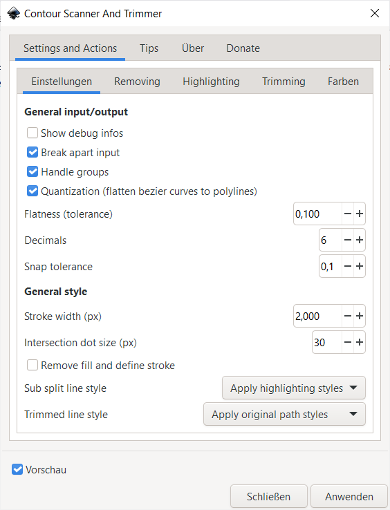
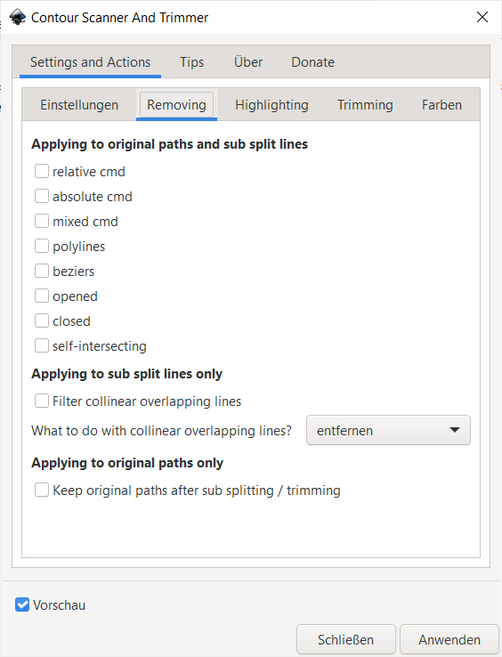
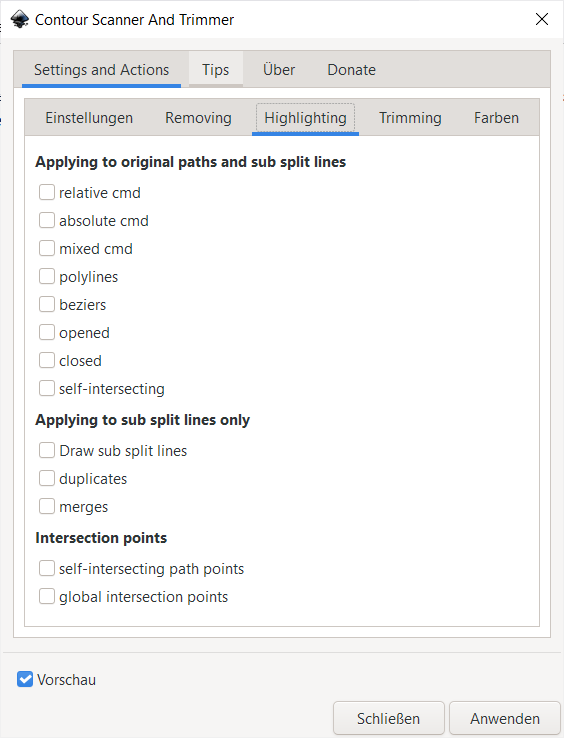
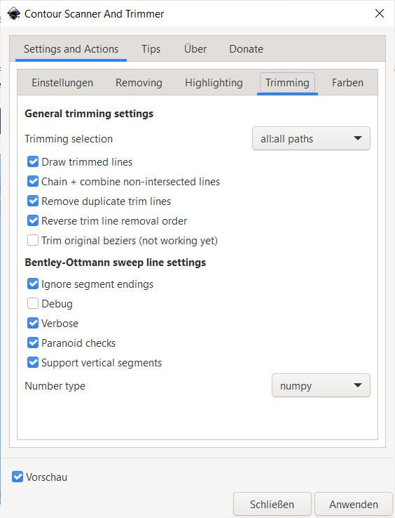
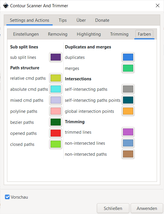
The user interface

Quick example

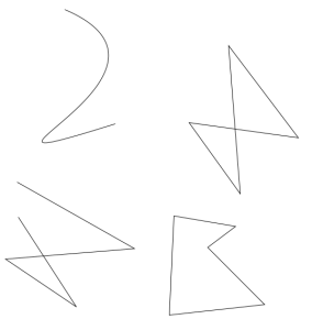
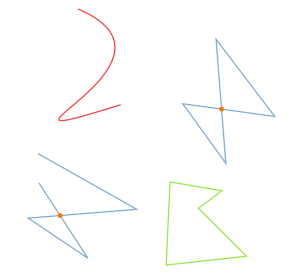
Using Contour Scanner and Trimmer we can check the different contours and their behaviour. Usually a contour can be open or closed and it can intersect with itself or not. This will give us 4 different combinations and we can use this information to find out where the intersections are using Bentley-Ottmann algorithm. Short examples:

4 different basic line "types"	Marked paths by running the extension using colors and dot modifiers

Real example

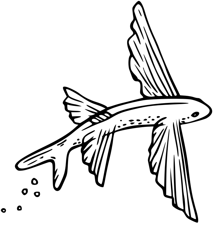
Load sove graphic you want to fix

Depending on the steps you want to perform with the file maybe create some duplicate.

Run the extension

Configure the setting depending on what you want.

Fix the desired paths

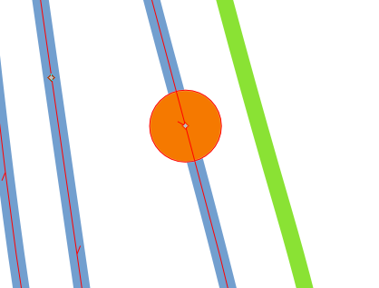
Select the path to see the handles. The dot indicates that there might be something faulty. In the following example there are two handles at the same coordinate. We can pick one of them to drag it away from the other one. You can now delete the marking point

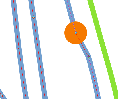
After rerunning the extension the dot will not appear again:

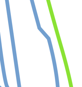
Overlapping lines

Contour Scanner is powerful. It can find and merge overlapping lines in the set of flattened sub split lines. We find those line intersections between lines where the same slope exists and which cover each other fully or partially (collinear overlapping lines). See the graphic to understand the problem.

At the moment Contour Scanner cannot remove those overlaps in original paths.

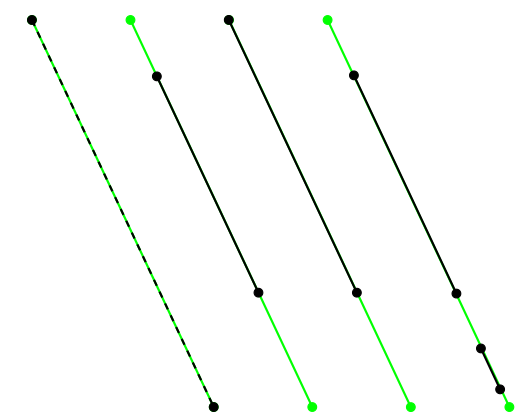
From left to right:

• 1st: path 1 is equal to path 2 (they share start point and end point and have the same direction)
• 2nd: path 1 and path 2 share direction, but not the start or end points
• 3rd: path 1 and path 2 share one point and direction
• 4rd: multiple overlapping lones

Issues

Trimming bezier curves

There is no algorithm done to split the original bezier curve after finding intersection points and t parameters yet.

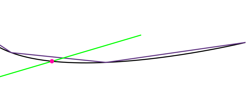
• green = a cutting line
• black = original bezier curve
• purple = approximated polyline
• magenta = intersection point between cutting line and original path (the intersection between cutting line and approximated curve would be far away as you can see)